Frequently Asked Rhetorical Questions (FARQ) about MUSSELp Cladomics Pages
What is cladomics?
Cladomics is a relatively new feature of the MUSSEL Project Web Site (since 2021). Cladomics is the branch of biodiversity informatics concerned with the study of cladomes — i.e., the set of all published species-trees/clades representing a taxon. For this site, the cladome refers to the set of clades among the available phylogenetic studies relevant to valid (i.e., currently recognized) freshwater mussel genera and family-group level taxa.
What are the data that are the basis for the MUSSELp cladomics pages?
We maintain a database of the branching topologies of phylogenetic trees with freshwater mussel taxa represented among the terminals. (Other taxa may be incidentally represented as well, but the intention at the time of this typing is to capture data on freshwater mussels.) A cladogram (= phylogenetic tree) is recognized by its unique combination of a publication code and a figure number from that publication. A publication may have multiple cladograms.
Each terminal or internal node is assigned a globally unique key (clade_id). The tree topology is stored as a list of nodes and the parent node from which each descends. The root of the tree is simply the deepest node lacking a parent.
Each terminal node is assigned a corresponding unique identifier of the nominal species or nominal genus in the MUSSELp database. Thus, as taxonomy is updated, the taxonomy of the cladograms is updated as well.
What software is used to handle cladomic data?
The data are captured and managed in FileMaker Pro Advanced, like the MUSSELpdb generally. For analyses, the data fields are exported as tab-delimited text, and custom Python 3.x.x and R 4.x.x scripts are used to manipulate and analyze tree topologies and make the cladomic reports for each taxon.
What information is presented in the cladomics report associated with a particular taxon?
The objective at this time is to list the topologies relevant to the focal genus, tribe, subfamily, etc. in question and the publications that report those topologies. These are sorted according to relevance.
For any genus or family-group level taxon to have a cladome to report, there must be a cladogram (i.e., a figure in a publication) that included at least one species classified in that taxon according to the MUSSELpdb. The species-tree topology is depicted for the taxon plus up to two more nodes — provided the nodes represent rigorous outgroups (see below). When a tree isn’t shown, it is because there is no in-group topology (e.g., 1 taxon) and the outgroups are too distantly related to be relevant.
Among the ingroup cladograms that are known for each taxon that have at least two representative ingroup terminal taxa, the proportion of cladograms that recovered the ingroup as monophyletic is reported.
Huh?
Consider the Lampsilini in Graf & Cummings (2006).
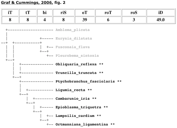
In the cladogram depicted in Fig. 2 of that study, to find the node/clade that represents that tribe, it is simply a matter of 1) analyzing all the clades with terminal taxa classified in the Lampsilini, and 2) finding the clade in that set that has all the lampsiline terminals in the analysis but the minimum number of total terminals. Graf & Cummings (2006) included 8 lampsiline species (in 8 genera) and they were recovered as monophyletic — there is a clade with all eight terminals and only those terminals.
That clade is shown, along with outgroup (non-lampsiline) branches. Only rigorous outgroup branches are shown. A rigorous outgroup is a terminal taxon classified in the same parent-taxon as the taxon in question. In this case, rigorous outgroups of the Lampsilini include any non-lampsiline terminals also classified in Ambleminae.
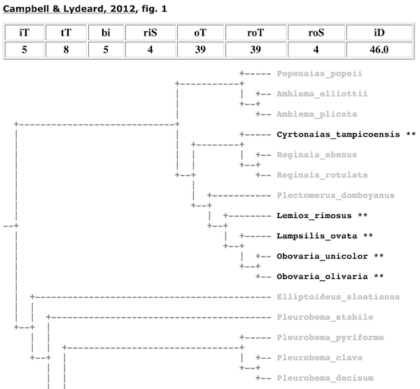
If a taxon is not recovered as monophyletic, the total clade size will be greater than the number of ingroup species. For example, Fig. 1 in Campbell & Lydeard (2012) does not depict the Lampsilini as monophyletic because the smallest clade that included five of the lampsilines species (in four genera) that were analyzed also contained non-lampsiline outgroup taxa.
Just do that for all the cladograms and all the genera and family-group level taxa — that will find the cladome for each supra-specific taxon. If you are interested in the phylogenetic evidence supporting the recognition of a particular taxon, the cladomics pages list the relevant publications and a preview of the various tree topologies. This links to publications and cladogram figures will take you to more information, including the entire species-tree.
By what criteria are the data sorted?
The clades are sorted primarily according to the number of ingroup terminals that were included in each publication: from most to the fewest.
However, the top publications are those deemed — by a so-far-pretty-primitive algorithm — to have provided the most robust tests of monophyly and sister relationships. These determinations are based on multiple criteria, using statistics to compare cladogram ingroup and outgroup sampling. If you are interested in the phylogenetic evidence supporting the recognition of a particular taxon and you only want to look up one or two papers, then the ones at the top are (hopefully) the go-to papers. (All the references are hot-linked to their publication page on this web site, which will link to the publication itself, if the URL is available.)
What statistics are used to compare cladograms?
Various criteria are used to evaluate and sort the cladograms. The data for each cladogram is provided in a table with eight columns: iT, tT, bi, riS, oT, roT, roS, and iD.
Ingroup Terminals (iT). — This refers to the number of terminal taxa representing the ingroup taxon in the cladogram. More ingroup terminals provide a more rigorous test of ingroup monophyly.
Total Terminals (tT). — Once the algorithm has determined the node that represents the most recent common ancestor of the ingroup, tT refers to the total number of terminal taxa in the clade. The ratio of iT to tT is used to determine monophyly. If iT/tT = 1, then the taxon was recovered as monophyletic. In the case of the Campbell & Lydeard (2012) tree above, the Lampsilini was not recovered as monophyletic since iT = 5, tT = 8, and iT/tT < 1.
Bipartitions (bi). — Within the ingroup clade, the number of bipartitions simply refers to the number of internal nodes. The number of bipartitions is an indication of how well-resolved the ingroup branches are.
Rigorous Ingroup Subtaxa (riS). — A rigorous test of monophyly will sample widely from the various subtaxa of the ingroup taxon. In the case of the tribe Lampsilini, the more genera sampled the better; for the subfamily Ambleminae, the more tribes the better, etc. The number of Rigorous Monophyly Subtaxa refers to the number subtaxa that are represented by iT. For example, in Graf & Cummings (2006), the 8 iT species represent 8 riS genera.
Outgroup Terminals (oT). — The rest of the terminal taxa in the whole cladogram that are not part of iT. More outgroup terminals provide a stronger test of monophyly.
Rigorous Outgroup Terminals (roT). — These are outgroup terminals that are classified as part of the same parent-taxon of the ingroup. In the case of the Lampsilini, roT refers to the other terminals of the Ambleminae. Outgroup terminals that are distantly related (i.e., have little chance of disrupting ingroup monophyly or being actual sister groups) provide less rigorous tests of monophyly and taxonomic placement than more closely related outgorups do.
Rigorous Outgroup Subtaxa (roS). — roS refers to the number of taxa of the same rank as the ingroup taxon represented in roT. Continuing the example of the Lampsilini, sampling from more of the other tribes of the Ambleminae provides a more rigorous test of monophyly that a less diverse array of outgroup terminals.
Ingroup Distance (iD). — The topology of each ingroup cladogram is compared with the top monophyly cladogram by pruning out terminals that are not shared in both. The algorithm also takes taxonomy into account by matching terminals that may represent higher taxonomic levels. Once the corresponding trees are found, the topological differences are quantified using the Robinson-Foulds metric. The iD is calculated using both R-F & the number of pruned taxa. The higher the iD, the more different the cladogram is from the top one.
The Robinson-Foulds metric (Robinson & Foulds, 1981) measures the distance between two cladograms as the sum of the unique biparititions in the two trees. Any tree can be split on any branch into two trees. Each subtree contains a mutually exclusive subset of the terminal taxa — a bipartition. It is simply a matter of finding all the bipartitions for the two cladograms, making a list of all the bipartitions that occur in one cladogram but not the other, and counting the elements of that list.
How can the Ingroup Distance (iD) be used to compare cladograms with different sets of terminal taxa?
When comparing cladograms with different sets of terminals, the "corresponding trees" need to be found first. This process involves pruning out taxa that are not shared between the two cladograms but also aligning different terminal species that might represent the same genus or higher taxon.
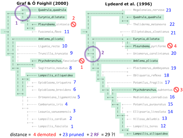
Consider, for example, the Ambleminae cladograms from the phylogenies published by Graf & Ó Foighil (2000) and Lydeard et al. (1996).
There are six terminals that are shared between the two cladograms (highlighted in green). However, two on each cladogram correspond at the genus-level: Pleurobema and Ptychobranchus are represented by different species. Four total terminals (marked in red) need to be demoted to a less specific rank — in this case genus. Twenty-three total taxa need to be pruned (blue).
The resulting corresponding trees represent all the shared species, genera, tribes, etc. of the two trees. The two corresponding trees also differ in topology, with each tree depicting a unique bipartition not shown in the other tree (purple).
The total Ingroup Distance (iD) of the Ambleminae on these two cladograms could be estimated as the sum of all the differences: 4 + 23 + 2 = 29, for example. These different distance metrics can be weighted in different ways, and we are still playing around with that.
Why do the terminal taxa in the cladograms sometimes look different from what the original authors reported?
For example, one of the terminals in Graf & Ó Foighil (2000) above is labeled "Sagittunio nasutus," but Sagittunio was not even described as a genus until 2018.
In that case, the taxonomy has been updated since the original publication. The objective is to report the taxa as they are currently recognized, not just as the authors reported them. This includes not only nomenclatural updates, but subsequent lumping and splitting, as well as re-identifications.
Also, since the goal is to report relationships among taxa rather than DNA sequences — i.e., species trees, not just trees of Genbank sequences. Any clade in the original tree with all terminals classified as the same species are collapsed down to a single terminal node.
In the cladomics reports, all terminals are collapsed down to rigorous ingroup and outgroup taxa. Thus, for the Graf & Cummings (2006) analysis of the tribe Lampsilini (shown above), the ingroup is shown as genera and the outgroup is represented by tribes. When rigorous ingroup and outgroup taxa can not be collapsed because they are not monophyletic, they still collapsed to the next lowest available level. This can be see, for example, in the the cladogram for the Lampsilini from Campbell & Lydeard (2012) (shown above).
In addition, it is sometimes the case that analyses were rooted in the original publication in ways that could be improved. Those improvements may be presented on this web site.
What is represented in the PCoA ordinations and NJ trees of pairwise ingroup distances?
For all the clades of the cladome of a particular taxon, the Ingroup Distance (iD) are calculated for every pair of cladograms with at least three taxa (i.e., one internal node). This distances are graphed using two different methods to depict the patterns of similarity among the clades of the cladome. They are pictures of the cladome.
Principal coordinates analysis ordination (AKA classical multidimensional scaling) is implement in base R and plotted with ggplot2, using the first two eigenvectors as the x- and y-axes.
A neighbor joining tree is draw with the R package APE using the same distance matrix as was applied to the PCoA.
For both graphs, each cladogram is represented by the combination of the unique publication code and the figure number of the published cladogram. Publication codes are provided with each publication heading in the list of cladograms.
These distance data probably violate important assumptions of these graphing methods, but right now, they are regarded as cool enough to be better than not having them.
What if I am really geeked-up about this and I have more questions?
Send an email to Prof. Daniel Graf in the Department of Biology at the University of Wisconsin-Stevens Point. There is a link to his home page (with contact information) in the footer of this web page. |